How to evaluate tracking with the HOTA metrics

How to evaluate tracking with the HOTA metrics

HOTA (Higher Order Tracking Accuracy) is a novel metric for evaluating multi-object tracking (MOT) performance. It is designed to overcome many of the limitations of previous metrics such as MOTA, IDF1 and Track mAP.

This short blog post gives an overview of the most important aspects of HOTA in three parts:

1. How to calculate the HOTA metrics.
2. How to compare trackers with the HOTA metrics.
3. How does HOTA compare to alternative tracking metrics.

For more details on HOTA, check out the IJCV 2020 paper and the metrics code on GitHub.

Part 1: How to calculate the HOTA metrics.

HOTA can be thought of as a combination of three IoU scores. It divides the task of evaluating tracking into three subtasks (detection, association and localization), and calculates a score for each using an IoU (intersection over union) formulation (also known as a Jaccard Index). It then combines these three IoU scores for each subtask into the final HOTA score.

Below we look at how the IoU score is calculated for each of these three subtasks.

Localization:

Localization measures the spatial alignment between one predicted detection and one ground-truth detection. Localization IoU (Loc-IoU) is typically used in many evaluation metrics to measure localization accuracy. It is calculated as the ratio of the overlap (intersection) between the two detections and the total area covered by both of them (union). This can be seen in the diagram below.

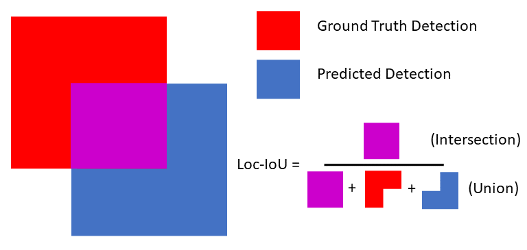
This concept trivially extends from bounding boxes to segmentation masks. As can be seen, when the Loc-IoU score here increases, the predicted and ground-truth detections are better spatially aligned and the localization is improved.

We can measure the overall Localization Accuracy (LocA) by averaging the Loc-IoU over all pairs of matching predicted and ground-truth detections in the whole dataset (we describe below how we obtain these matches):

Detection:

Detection measures the alignment between the set of all predicted detections and the set of all ground-truth detections. Detection IoU (Det-IoU) is also commonly used for measuring detection accuracy. Here we need to define which detections between the set of predicted and ground-truth detections are intersecting. To do this, we define a localization threshold (e.g. Loc-IoU > 0.5) above which we say that two detections intersect. However one predicted detection may overlap with more than one ground-truth detection (and vice-versa). To deal with this we run the Hungarian algorithm to determine a one-to-one matching between predicted and ground-truth detections. These matching pairs of detections are called True Positives (TP), and can be thought of as the intersection between the two sets of detections. Predicted detections that don’t match are False Positives (FP) and ground-truth detections that don’t match are False Negatives (FN). The detection IoU is then given by:

We can see that this has fundamentally the same structure as Loc-IoU. It is the intersecting area (the matches or TPs) divided by the total area (the union over all detections). Whereas Loc-IoU measures the alignment between a single predicted and ground-truth detection, the Det-IoU now measures the alignment between the set of all predicted detections and the set of all ground-truth detections. This set-based IoU formulation is also commonly called a Jaccard Index.

We can measure the overall Detection Accuracy (DetA) by simply calculating the Det-IoU using the count of TPs, FNs and FPs over the whole dataset:

Association:

Association measures how well a tracker links detections over time into the same identities (IDs), given the ground-truth set of identity links in the ground-truth tracks. We can measure this by taking a predicted detection and ground-truth detection that are matched together (using the Hungarian matching as explained above), and measuring the alignment between this predicted detection’s whole track and the ground-truth detection’s whole track. This alignment can again be represented in an IoU formulation.

The intersection between two tracks can be measured as the number of True Positive matches between the two tracks, we call these True Positive Associations (TPA). Any remaining detections in the predicted track (which are either matched to other ground-truth tracks or none at all) are False Positive Associations (FPA) and any remaining detections in the ground-truth track False Negative Associations (FNA). The Association IoU (Ass-IoU) can then be calculated in a similar way as seen previously:

This now measures the alignment between two tracks, which gives us a measure for every pair of matching detections (TPs) how good the association is for this detection.

We can see a visual example of the definitions TPA, FNA and FPA below:

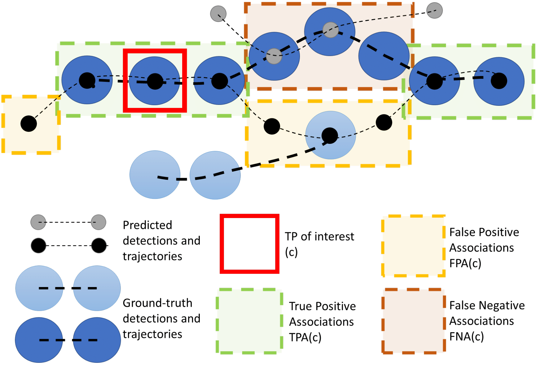
The red square indicates the matched TP pair of a prediction and ground-truth detection, for which we want to find an association score. In order to measure how good the temporal association aligns between these detections, we find all the detections in these two tracks which match between these tracks (TPAs in green) and all the detections where they don’t match (FPAs in yellow and FNAs in brown).

We can measure the overall Association Accuracy (AssA) by averaging the Ass-IoU over all pairs of matching predicted and ground-truth detections in the whole dataset:

Building HOTA from three different IoU scores:

Naturally, all three components (localization, detection and association) are important for tracking success, so it’s important to measure all of them. However, we often want a single metric which we can use for ranking how well trackers perform overall. This metric is HOTA, which is a combination of all three IoU scores defined above:

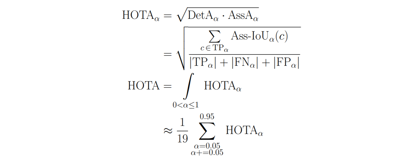
Note that earlier, both the DetA and AssA were defined using a Hungarian matching based on a certain Loc-IoU threshold (α). Since the DetA and AssA score both depend on the Loc-IoU values, we calculate these score over a range of different α thresholds. For each threshold value, we calculate the final score as the geometric mean of the detection score and the association score. By then integrating over the different α thresholds, we include the localization accuracy into the final score.

The use of the geometric mean for combining detection and association ensures that both are evenly weighted in the final score, and that the score goes to 0 if either detection or association go to zero. Furthermore, this has the interpretation that the HOTA score can be thought of as a Det-IoU formulation where each of the TPs in the numerator are weighted by the Ass-IoU for this TP. E.g. an average of the Ass-IoU scores over the union of all detections.

Part 2: How to compare trackers with the HOTA metrics.

Armed with the family of HOTA metrics, we can now evaluate multi-object tracking in way that was not possible before. We can now not only see how good a tracker is, but also where it is good, which is crucial for understanding the underlying behavior of a tracker when both deciding on a tracker for an application, and when investigating how to improve current trackers.

As an example, let’s look at the results of the top 20 methods (as of when this was written) on the KITTI tracking leaderboard for pedestrians:

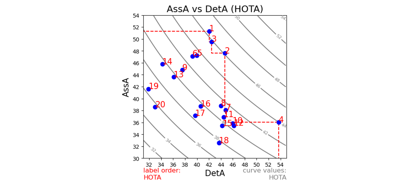
The rank (red number) gives the order of the methods, ordered by the overall HOTA score. However, now we can see how well methods perform in each of the dimensions of detection (x-axis) and association (y-axis) separately, with the curves in the background showing how the overall HOTA score increases as both detection and association scores increase.

The top 3 ranked trackers have a very similar overall HOTA scores (46.3%, 45.9% and 45.7%), but we can see from this plot that there is a clear difference in where one is better than the other. Tracker 1 is the best at association, while Tracker 2 is better at detection and Tracker 3 is in between the two for both. If you wanted to select a tracker for a particular application, you could now decide whether association or detection was more important for your application and pick the most appropriate tracker accordingly. In fact, each of these three trackers lie on the Pareto optimal front (red dashed line) such that for some level of trade-off between association and detection accuracy each is the best choice. With the HOTA metrics there is now not only a single best tracker at the top of the leaderboard, but rather a number of best trackers with different trade-offs along the Pareto optimal front (Hat tip to Jack Valmadre and Alex Bewley for the idea of plotting Pareto fronts).

If the author of Tracker 2 wishes to improve his tracker, these results now indicate that he can improve it by looking into how Tracker 1 performs association, while in contrast the author of Tracker 1 might want to look into how Tracker 2 (or better Tracker 4) performs detection.

We can go further than just comparing detection and association. Because each are designed using an IoU formulation, they are both naturally decomposable into one component that only measures recall, and one component that only measures precision. We can perform this decomposition and plot the results to get even further insight into the tracking results:

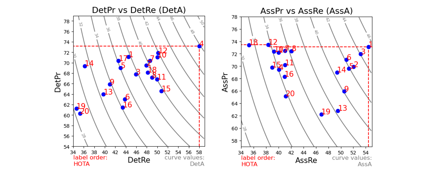
The above plots have tracker numbers ordered by the overall HOTA score still, so the same number refers to the same tracker as above. Detection recall (DetRe) measures how well a tracker finds all the ground-truth detections, whereas detection precision (DetPr) measures how well a tracker manages to not predict extra detections that aren’t there. From the first plot above, we can see that Tracker 1 and Tracker 3 have a similar detection accuracy overall, but Tracker 3 generally finds more of the ground-truth objects (higher recall), but also predicts more detections that are wrong (lower precision).

Precision and recall are commonly used for evaluating detection, but now with the HOTA metrics we can extend these concepts to also measure association. Association recall (AssRe) measures how well trackers can avoid splitting the same object into multiple shorter tracks. In contrast, association precision (AssPr) measures how well tracks can avoid merging multiple objects together into a single track. E.g. Tracker 15 is more likely to split tracks into multiple smaller ones than tracker 20, but it is better at not merging tracks together. Like detection precision and recall, there is a natural trade-off between association precision and recall when designing trackers.

The HOTA metrics allows meaningful analysis and comparison between trackers over all four of these dimensions (missing detections, extra detections, splitting tracks and merging tracks) while also combining all of these scores meaningfully into an overall score for ranking trackers.

Finally, HOTA also allows the analysis of localization accuracy:

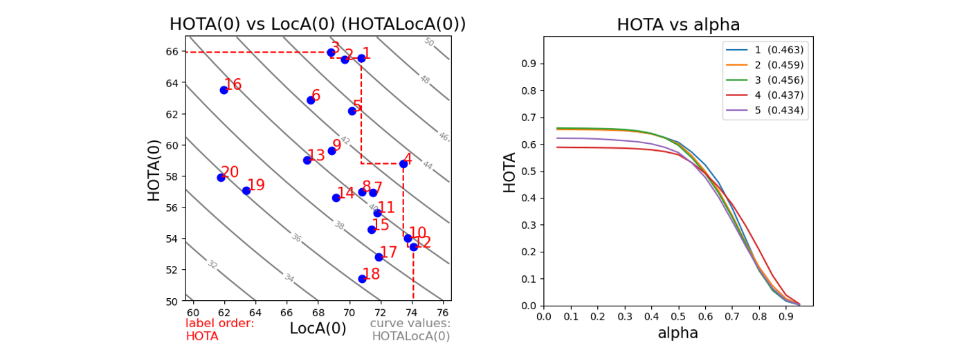
In the first plot above we compare HOTA(0) (HOTA at the single lowest alpha threshold, so to not include the influence of localization accuracy, in this case at alpha=0.05) against the localization accuracy LocA(0) (LocA at the same threshold). We can see that Tracker 3 performs slightly better than Tracker 1 at HOTA(0), e.g. when allowing detections to match even if they have only a little overlap, Tracker 3 has overall better detection + association, however the localization of these matched detections is worse, such that when we calculate the final HOTA score by calculating over the range of localization thresholds, Tracker 1 has a higher score. This shows how HOTA is able to decompose and combine tracker behavior not only for detection and association but also for localization.

In the second plot, we compare the top 5 trackers’ HOTA scores across the range of different alpha thresholds. All trackers get worse when increasing the alpha threshold, but the rate at which they get worse is interesting and is useful for comparing behavior between trackers.

Part 3: How does HOTA compare to alternative tracking metrics.

Previously, three other main metrics have been used for evaluating multi-object tracking, these are MOTA, IDF1 and Track mAP. We won’t go into the details of each one here, but rather walk through a simple example which highlights the differences between HOTA and the previous metrics:

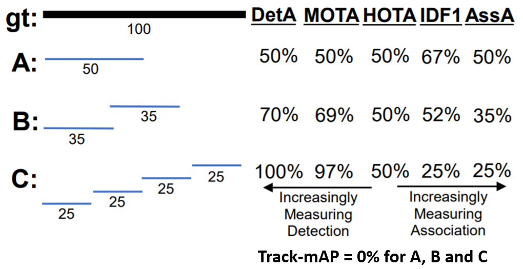
In this example, we have single ground-truth object, which is present in all frames of a 100 frame video. We then have three different trackers (A, B and C) with increasing detection accuracy and decreasing association accuracy. In this example, every predicted detection is a TP (e.g. matches with the ground-truth).

Which tracker is better out of A, B and C? This is not a well-defined question, because each tracker is very different, some are better at detection, others at associations, so it depends which of these are more important for your application. Since often both detection and association are very important, HOTA is designed to equally weight each of them in calculating an overall score. This can be seen in the above example. The detection score (DetA) increases, while the association score (AssA) decreases, such that for all three the combined HOTA score remains the same.

In comparison it can be seen that the MOTA score is heavily biased towards measuring detection at the expense of ignoring association. In contrast the IDF1 score is heavily biased towards measuring association, at the expense of ignoring detection. HOTA finds a perfect balance between these two extremes by equally weighting both detection and association, while allowing analysis of each component separately with the DetA and AssA sub-scores.

Finally the Track mAP metric is the least informative of all the metrics in our example because it requires predicted tracks to have more than 50% overlap with ground-truth tracks to count at all. Thus all three trackers in our example have a Track mAP score of 0, as if the tracker didn’t run at all.

Summary:

In this short blog post we’ve introduced the HOTA metrics, a new family of metrics for evaluating multi-object tracking. We’ve walked through how HOTA is calculated as the combination of three separate IoU scores for detection, association and localization respectively. We’ve seen how we can evaluate and analyze trackers along these different dimensions using different HOTA sub-metrics, and how each of these can be split into a recall and precision component for more fine-grained analysis. Finally we’ve briefly seen how these HOTA metrics compare with other metrics previously used for multi-object tracking evaluation, and highlighted some of the reason why using HOTA is often preferable.

For more details on HOTA, check out the IJCV 2020 paper (especially for detailed comparison and analysis between different metrics) and the metrics code on GitHub. This code can be used to evaluate your own trackers with HOTA, while also providing all of the analysis and plots in this article. Code is also present for other metrics for easy comparison, and it is easy to add new benchmarks and new metrics. HOTA metrics is currently rolling out to a number of different tracking benchmarks, check the GitHub readme for updates.

@article{luiten2020IJCV,
  title={HOTA: A Higher Order Metric for Evaluating Multi-Object Tracking},
  author={Luiten, Jonathon and Osep, Aljosa and Dendorfer, Patrick and Torr, Philip and Geiger, Andreas and Leal-Taix{\'e}, Laura and Leibe, Bastian},
  journal={International Journal of Computer Vision},
  pages={1--31},
  year={2020},
  publisher={Springer}
}