Differentiable Volumetric Rendering

Deep neural networks have revolutionized computer vision over the last decade. They excel in 2D-based vision tasks such as object detection, optical flow prediction, or semantic segmentation.

_{Image Source: Wayve.ai}

However, our world is not two- but three-dimensional! If we think about self-driving cars as an example, we can see that autonomous agents need to understand our 3D world to safely interact and navigate in it. They need to reason in 3D.

In our previous project Occupancy Networks we asked ourselves: “How should we represent 3D geometry in learning-based systems?” It turns out that using implicit neural function representations for 3D geometry is promising and has various advantages over previous representations. For example, implicit representations do not require discretization of the 3D space (e.g. into voxels or points) and are able to represent 3D shapes at arbitrary precision.

The Challenge

While this works well for synthetic data, we also like to scale to real-world scenes: However, existing approaches require 3D supervision. This means that during training, we need pairs of images and corresponding 3D objects. While 3D geometry is readily available for synthetic objects, it is typically hard to acquire in the real world or requires expensive and bulky laser scanning equipment. Therefore, in our recent work Differentiable Volumetric Rendering, we investigate how we can infer implicit 3D representations without 3D supervision by training them from ordinary 2D photographs.

But how do we do it?

Our Approach

First, let’s have a look at how we represent textured objects. We define two functions, an occupancy network \(f_\theta: \mathbb R^3 \to [0, 1]\) which assigns an occupancy probability to every point in 3D space. The 3D geometry of an object is then implicitly given as the decision boundary of this binary classifier. We further use a texture field \(\mathbf{t_\theta}: \mathbb R^3 \to \mathbb R^3\) which assigns an RGB color value to every point in space. We implement both $f_\theta$ and $\mathbf{t_\theta}$ in a single neural network with two shallow heads.

How do we render an image of a 3D shape?

If we want to train our network with 2D-based observations like RGB images or depth maps, we need to render our representation. Rendering refers to the process of obtaining images from a 3D representation. If we can realize this rendering operator we can then later manipulate the 3D structure such that the rendered image conforms to the 2D photographs we have taken from the object. To render a 3D structure into a 2D image, we first cast a ray from the camera to pixels and evaluate equally-spaced points on this ray. Next, we find the interval where points change from being outside ($f_\theta(\mathbf{p_j}) < 0.5$) to inside the object ($f_\theta(\mathbf{p_{j+1}}) > 0.5$). Using a root-finding algorithm, e.g. the Secant method, we obtain our final depth prediction. But how do we get the RGB values?

Using our predicted depth map, we can now unproject a pixel $\mathbf{u}$ back into 3D space to $\mathbf{\hat p}$. We simply evaluate our texture field at this point which gives us our predicted RGB color value $\mathbf{t_\theta}(\mathbf{\hat p})$!

How do we get the gradients?

For training a deep model, we need to infer the parameters of the model using gradient-based techniques such as stochastic gradient descent. Thus, we have to calculate gradients of the rendered image with respect to the model parameters $\theta$.

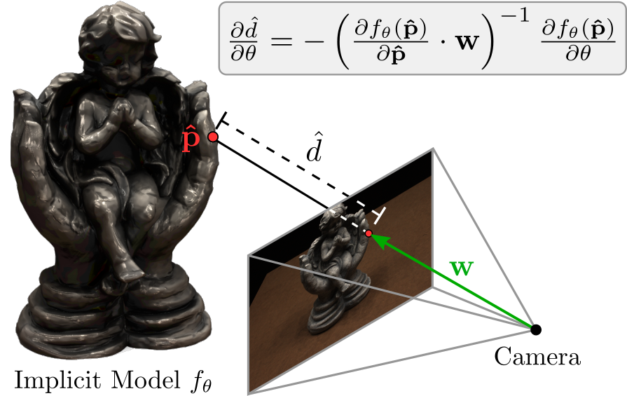
We find that we can derive an analytic expression for the gradient of the depth with respect to the network parameters $\theta$. We first observe that we can express the point on the surface as $\mathbf{\hat p} = \mathbf{r_0} + \hat{d} \mathbf{w}$ where $\mathbf{r_0}$ is the camera origin, $\mathbf{w}$ the ray to the pixel and $\hat{d}$ the predicted depth. But we also know that our surface is defined as the decision boundary of our occupancy network! Hence $f_\theta(\mathbf{\hat p}) = 0.5$. When we differentiate both sides for $\theta$ and insert the first formula into the second one, we obtain

\[\frac{\partial \hat{d}}{\partial \theta} = - \left( \frac{\partial f_\theta(\mathbf{\hat p})}{\partial \mathbf{\hat p}} \right)^{-1} \frac{\partial f_\theta(\mathbf{\hat p})}{\partial \theta}\]

We have found a way to calculate the gradient for the depth with respect to the network parameters analytically. This is great as we do not need to approximate the backward pass nor do we need to save intermediate results as for voxel-based rendering approaches!

Does it work?

We find that we can infer accurate 3D geometry and texture from a single image although we only train with 2D (RGB Images) or 2.5D (RGB Images + Depth Maps) supervision!

We further observe that we can use our model for real-world multi-view reconstruction. We obtain accurate shape, normal, and texture for this real-world example.

Further Information

To learn more about Differentiable Volumetric Rendering, watch our video here:

For more detailed information, check out the paper and supplementary. You can further have a look at our animated slides and if you are interested in experimenting with DVR yourself, download the source code of our project and run the examples. We are happy to receive your feedback!

@inproceedings{Niemeyer2020CVPR,
    title = {Differentiable Volumetric Rendering: Learning Implicit 3D Representations without 3D Supervision},
    author = {Niemeyer, Michael and Mescheder, Lars and Oechsle, Michael and Geiger, Andreas},
    booktitle = { Proceedings IEEE Conf. on Computer Vision and Pattern Recognition (CVPR)},
    year = {2020}
}